Representing 3D Models
December 19, 2022
In this post, I wanted to write out some notes based on my recent attempts to better understand how 3D models are stored and used for rendering. The focus here is mostly on unexpected findings or ideas that are obvious in hindsight, but I had never stopped to consider.
Real vertices
Below, we have a UV plot and 3D plot of a triangular pyramid. The UV plot is a mapping showing how 2D texturing data is applied to the 3D model. In this case, you can imagine the UV plot as if it was a 2D piece of paper that you could fold up to get the 3D model (a.k.a a net). In case the 3D plot below isn’t clear, you can click and rotate it to get a better sense of the shape. How many vertices would you say the pyramid has?
From the 3D plot, we see that the geometry of the pyramid requires 4 vertices to represent: 3 for the triangular base and 1 for the pointy tip. But when we look at the UV plot, we count 6 vertices! Intuitively, it seems like these aren’t the real vertices, for example, some of the 6 UV vertices represent the same physical location. Specifically, the 3 corner UV vertices all correspond to the tip of the pyramid.

Now imagine we were trying to communicate this pyramid model to somebody else so that they could load and render it themselves, how would we store the data? If we insist that there are only 4 real vertices in the model, then it makes sense to describe the model in terms of these 4 vertices. For example, we might list out each of the vertices along with their (X, Y, Z) coordinate:

This representation is a good start, but it doesn’t say how these points are connected, so we still need to describe how to form the faces of the pyramid. We can do this by listing the vertices that should be connected to form each face. For example, we can see that the base of the pyramid is formed by connecting vertex 1 to vertex 2 and then to vertex 3 (and back to vertex 1, though we can assume that we always connect the first & last vertices). More compactly, we could say something like: Face 1: [1, 2, 3] to describe the base of the pyramid. We can repeat this for the other faces and add them to our model definition so far:
We’ve done enough here to define the geometry of the pyramid, but we still need to encode the UV coordinates so that textures could be applied to the model. Clearly, we now need more than just the XYZ position listed for each vertex. Earlier we insisted that there should only be 4 vertices, so to avoid adding new vertex entries, we’d need to nest the UV data under the existing entries…
But we can already see a problem developing here. Earlier we noted that of the 6 UV coordinates, 3 of them correspond to the same XYZ coordinate (the tip of pyramid). In our current representation, this means we need to be able to store more than one UV entry for some of the vertices. We’d end up with something like the following:
By adding indexes to each UV entry (i.e. UV1, UV2, UV3), we’ve managed to encode the 6 unique UV coordinates with only 4 vertices. However now we’ve broken our face indexing, since it isn’t clear which UV entry we should pick if we only say to ‘connect vertex 1 to 2 etc.’. One obvious fix would be to expand on our original face encoding, so that we store a pair of indices, now representing the vertex and the corresponding UV entry. For example, the face representing the base of the pyramid (Face 1) would change as follows:
Previously we said that Face 1 was made by connecting:
Vertex 1 to vertex 2 to vertex 3
Our new representation says to connect:
Vertex 1 and it’s first UV entry, to vertex 2 and it’s first UV entry, to vertex 3 and it’s first UV entry
In this case we keep using the first UV entry, which makes sense since these vertices only have a single UV entry anyways, but we could reference other entries if needed. If we go ahead and repeat this process for the other faces, we get the following final representation:
This would actually work as a full representation of our pyramid, both the geometry and texturing information is fully specified! However, we’ve made a bit of a mess of it by insisting that there are only 4 vertices. For example, the indexing pairs used to define the faces are implicit. It’s not obvious that the first number in the pair (4,2), is meant to represent the XYZ value of the 4-th vertex entry, while the second number is an index into the 2nd UV entry nested under vertex 4 - those are two completely different kinds of index!
For such a simple model, our format works but it’s a bit unwieldy. What happens once we add normals, or vertex colors into this? If we really did try to communicate this model data to someone else, we would have to separately tell them how to interpret the face indexing to make sense of the UVs, normals, colors etc. Ideally this information would be part of the data itself.
So is there a better way to represent the data, or are 3D models just inherently messy complicated data structures? Well the popular .obj format uses an improved variant of our intuition-driven format. Here’s an example of the pyramid model encoded as a .obj file, in a slightly more structured form:
As we can see, the .obj-style format uses the same sort of ‘faces include multiple indices’ trick that we landed on earlier. However, there are some improvements. For one, the clear separation of XYZs and UVs means that the awkward nested UV indexing (i.e. ‘UV entry 2 of vertex 4’) is no longer a problem. Additionally, the ordering of the indices used by the faces is actually communicated by the order of appearance of the XYZs and UVs sections. For example, the pair (4,6) is interpreted as meaning:
Take the 4th entry from the first section (
XYZsin this case) and the 6th entry from the second section (UVsin this case)
If we were to add more data, like vertex coloring for example, that data could just be inserted below the UVs section and added as a 3rd index entry in the face data!
Ultimately, the improvements of the .obj format over our original format come from throwing away the idea that the model is made of 4 real vertices. Instead, this format is really describing the model as being made of 4 real faces. I had an oddly difficult time wrapping my head around this, but it does seem like the more intuitive interpretation. For example, while this model has different numbers of XYZ and UV points, it ends up having exactly 4 faces in both the UV and 3D visualizations and they have a direct correspondence. Rather than being the ‘real’ data, the vertex positions and UV coordinates can instead be thought of as a set of attributes associated with the points making up each face.
Interestingly, if we export this pyramid model as a .ply file from Blender, we get a very different representation than if we export a .obj! In fact Blender reports the model as having 6 unique vertices, 4 faces and nothing else. The 6 vertices are really coming from the UV map in this case, and the XYZ coordinates are just duplicated wherever neccessary. Here’s an example of the model encoded by Blender when exported as a .ply file, in a slightly more structured form:
Aside from using 0-indexing for the faces, the other big difference with the .ply export is that each vertex is represented as a 5-dimensional point: (X,Y,Z,U,V). Our pyramid isn’t made of 4 points in 3D space, it’s made of 6 points in 5D space, pretty cool! If we wanted to include vertex color data for example, we’d just add more dimensions to each vertex. By taking this approach, we’re able to avoid the need for complex indexing when describing the faces.

In many ways, the .ply formatting seems like a much simpler way to represent the model, though the fact that it duplicates some vertex positions may seem undesirable. It’s worth noting that this representation (as well as the .obj format) are meant for model storage and rendering, they wouldn’t be suitable for use in an editing context (i.e. direct manipulation by 3D artists). For one thing, they don’t explicitly represent the edges of the model, something that’s quite helpful to be able to access and modify for a 3D artist.
While the .ply formatting seems much cleaner, I actually think it’s slightly better to think of 3D models more like the .obj interpretation. The main reason for this is that the idea of building faces from a set of distinct attributes is closer to how rendering actually works in practice (from my limited experience at least).
Triangles everywhere all at once
Speaking of how rendering works, although the model representations allow for faces with any number of vertices, everything must eventually be converted to a triangle in order to render on screen (at least for conventional rasterized graphics, though there are alternative approaches). On the other hand, quads (i.e. polygons made of 4 points) are far more common to use when it comes to 3D modelling. One reason for this is that quads have an unambiguous directionality to them. If you imagine entering a quad from one of it’s edges, it’s clear which edge is opposite the one you entered: it’s the one that doesn’t share any vertices with the edge you entered through.


This makes it possible to specify a ‘line through a quad’, and then have the computer extend that line through all connected quads, leading to the concept of face loops and edge loops - very handy features for 3D modelling!

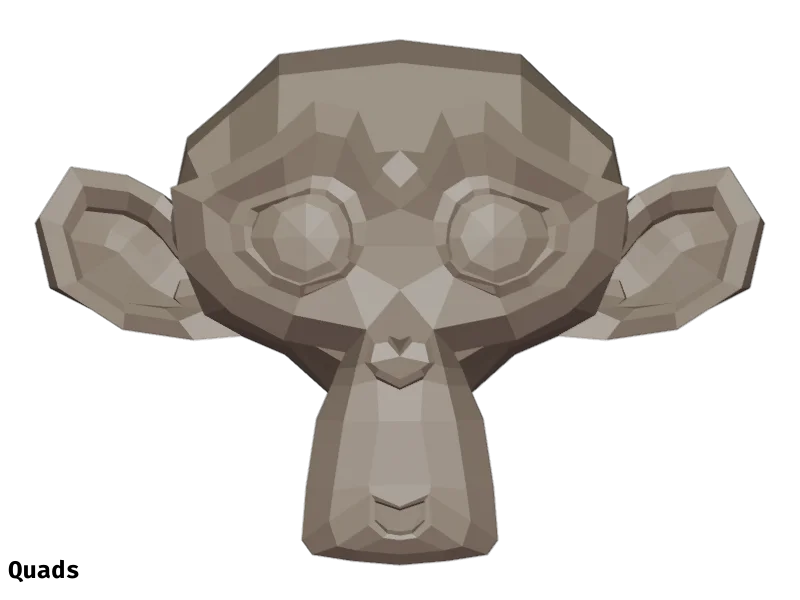
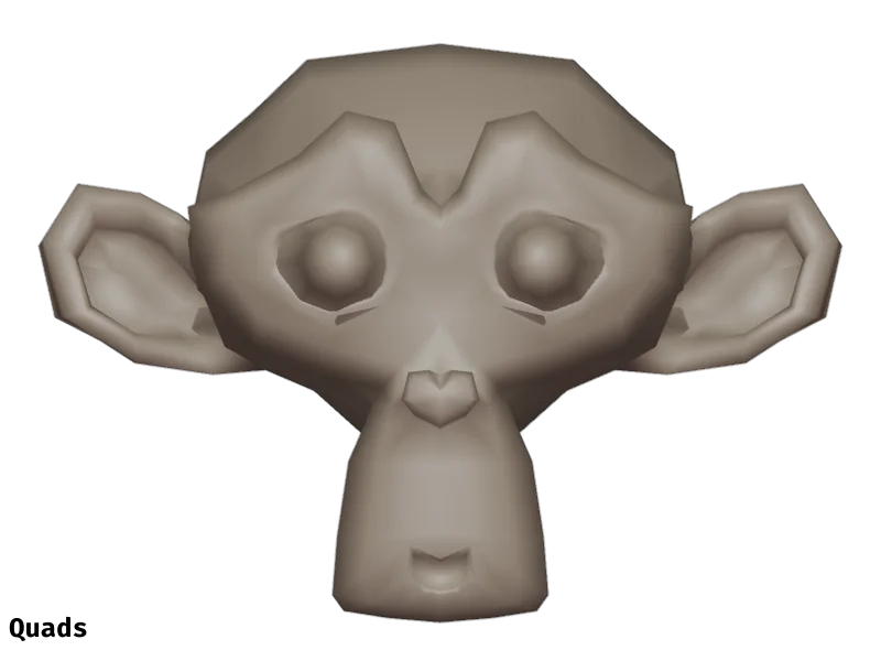
Due to the convenient features of using quads for 3D models, most models are likely authored and stored in terms of quads, in spite of the need for triangles when rendering. No problem though, a quad is just made of two triangles. When it comes time to render we just replace each quad with two triangles and the result is the same, right? To my surprise, this isn’t quite true! While we can replace any quad with two triangles, the resulting triangulated model is not equivalent in appearance (in general) to the original quad-based model. Part of the reason for this discrepancy is that there is a well defined way to calculate a single normal vector for a quad. For example, we can calculate the cross-product between the vectors connecting opposite corners of a quad to give us a vector perpendicular to the ‘surface’ of the quad, even if the surface isn’t actually flat! More generally, there’s a way to define normal vectors for any polygon, called Newell’s method, but I’m going to skip over that here.


However, while we can define a single normal vector for a quad, that same quad split into a pair of triangles may have two different normal vectors. So if the quad isn’t flat, it will have different shading depending on whether it is interpreted as a quad or as two triangles. When working in a 3D editor, you’re likely to see the quad interpretation. If you export a model to use somewhere else (like in a game engine) you’re likely to see the triangle interpretation.
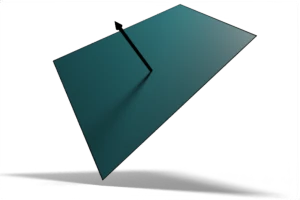
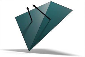
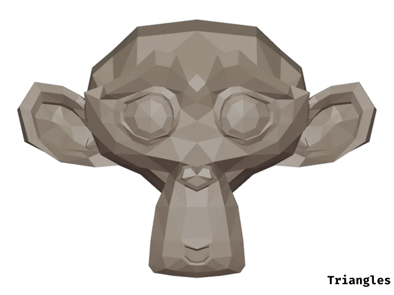
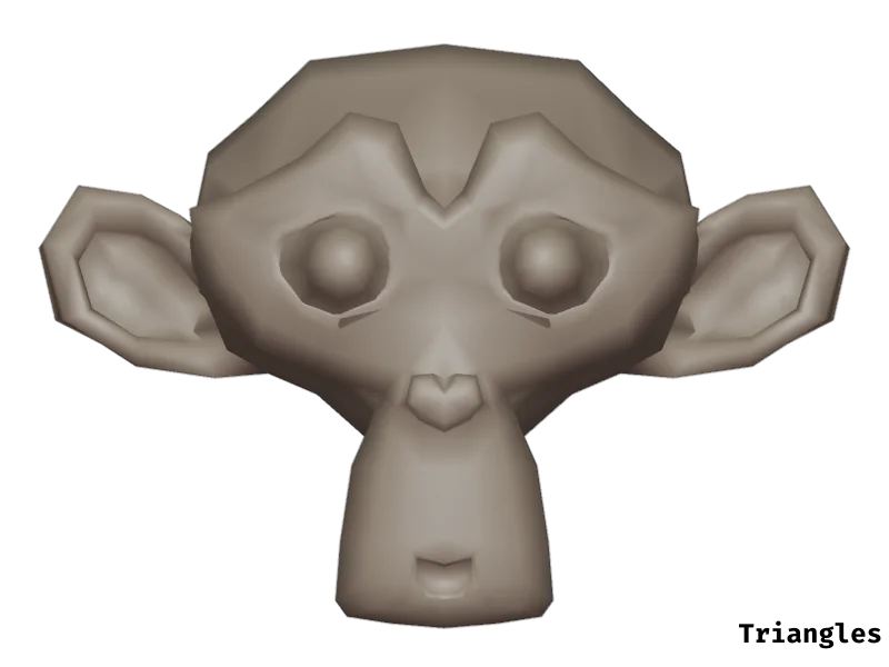
So is this a concern if you’re a 3D artist? Do you have to worry about the difference between your authored model and the triangulated version when rendering? I think if you were using flat/faceted shading, then yes it could be a problem - you’d want to make sure each quad is actually flat to avoid the uglier triangle shading (or otherwise use a renderer that supports face-based shading). For smooth shading, the differences are less noticable and the results from triangle shading may actually be preferred. An interactive comparison is shown below, using the Suzanne model from Blender. Quad shading is shown on the left side of the image, while triangle shading is shown on the right, click and drag to move the dividing line. As an example of how differently the shading can look, check out the upper eye socket area:
Sad normals
We just talked about normal vectors, which define the direction that a single face (a quad or triangle for example) is… facing. By comparison, a normal map is a special texture which can be used to provide information about a model’s surface normals within the faces of a model. These maps use the red, green and blue values of an image to encode the x, y and z components, respectively, of a normal vector at each point on the surface of a model, according to it’s UV map. This makes it possible to ‘fake’ intricate lighting and shadowing effects on the surface of a model, without requiring extremely dense geometry.
This is both a wildly clever trick and yet so common it’s also mundane and easy to take for granted once you’ve seen it a few times. Until recently, I had never considered that if a normal map is used to represent surface normals, why do they always look so blue? Surely the surface normals of most models end up pointing in all directions: some pointing mostly along the x (red) axis, some along the y (green) or z (blue) axis, others somewhere in-between. Yet a mostly blue normal map implies all the normals point along the z-axis, since blue-ness corresponds to the z-component of the vector.
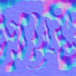
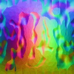
Clearly, these blue-ish normal maps aren’t encoding the absolute normal vector, but some kind of relative offset. This seems fairly obvious after spending some time thinking about it, but it’s yet another thing that caught me off guard when looking into 3D rendering, despite the fact that I thought I was already familiar with normal maps. That being said, I haven’t dealt with any of the implementation details of normals maps, so I don’t have much more to say here (like how do you actually generate the resulting normals? How do you even encode a relative offset for a normalized vector?).
I did find that there is such a thing as a normal map encoding absolute vectors, which is called an object space normal map. By comparison ‘normal’ normal maps (at least the ones I’m used to seeing) are more formally called tangent space normal maps. So why don’t we see object space maps as often? While there seem to be several reasons, the advantage that stands out the most is that tangent space maps can be used across many objects, since they aren’t tied to a specific geometry.